Batch or continuous distillation packages
Obtain the OEM’s process-facing duty, operating modes, ramp and utility interfaces. Compare the package’s real production pattern rather than averaging a peak over the whole day.
Coordinate specialist distillation packages with steam, cooling, condensate, controls and site interfaces before expanding utility capacity.
Start with the business outcome
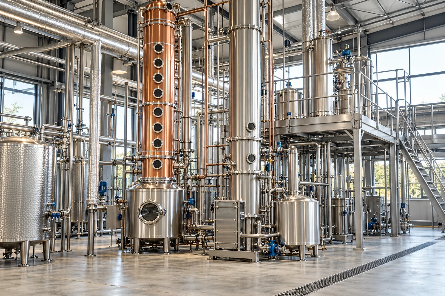
A distillery may need stable process-facing heat rather than a larger source alone. DPS can coordinate specialist distillation equipment with utility distribution, returns, controls and installation. The business case should use measured baseline energy / service changes and qualified operating duty. Production volume or alcohol strength cannot be inferred from an energy-saving percentage.
Qualified distillation OEMs and site specialists establish process performance, product specifications, pressure systems, hazardous-area requirements and applicable approvals. DPS integration does not imply manufacture of every still, column or specialist vapor system.
Obtain the OEM’s process-facing duty, operating modes, ramp and utility interfaces. Compare the package’s real production pattern rather than averaging a peak over the whole day.
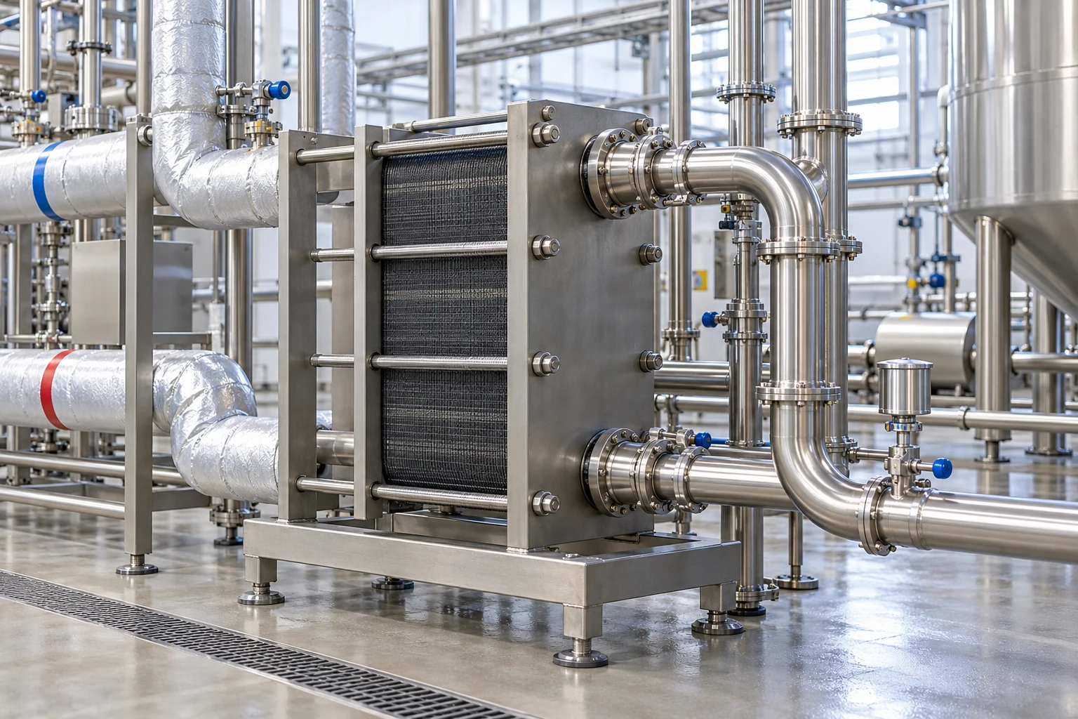
Inspect pressure control, trapping, drainage, returns and potential contamination pathways with qualified specialists. Recovery must preserve required utility / product quality.
Match supply / return conditions and concurrent demand to the package. Cooling limitations and heat rejection can restrict operation independently of steam availability.
Measure steam conditions at the user during representative distillation duty.
Compare recoverable duty, reuse destination and necessary quality / isolation boundaries.
Coordinate the package with steam, cooling, controls, structures and qualified site work.
Swipe horizontally to compare all columns ↔
| System | Operating duty | Relevant DPS guide | Confirm before purchase |
|---|---|---|---|
| Specialist distillation package | Perform the product-specific separation duty. | Process engineering ↗ | OEM process, pressure / vapor and qualified site responsibilities. |
| Utility supply and return | Meet the duty where the process actually uses it. | Utility infrastructure ↗ | Peak overlap, recovery, quality, point-of-use conditions and isolation. |
| Instrumentation and controls | Execute the agreed sequence and record meaningful equipment states. | Automation & controls ↗ | I/O, alarms, recipe authority, backups and acceptance tests. |
| OEM and field interfaces | Connect the selected equipment to the existing operating train. | Installation & integration ↗ | Mechanical, electrical, software, site access and integrated acceptance. |
The supplier’s historical case is independent of the example below. Compare your measured duty and all-in cost without adopting another site’s savings or payback.
Swipe horizontally to compare all columns ↔
| Decision | What to compare | Acceptance evidence |
|---|---|---|
| Additional source | Verified package heat demand and existing delivery | Required conditions across defined concurrent users. |
| Distribution / drainage correction | Local control, returns and restrictions | Stable package duty and measured cost change. |
| Recovery | Available heat, receiving load, timing and quality | Net avoided purchased energy after added operation. |
Swipe horizontally to compare all columns ↔
| Observed condition | Measure before design | DPS / team decision | Economic basis |
|---|---|---|---|
| Unstable delivered heat | Measure package conditions and return behavior. | Correct source / distribution / drainage duty. | Verified resource and maintenance costs. |
| Lost recoverable heat | Build a metered energy balance. | Compare suitable recovery destinations. | Actual baseline fuel / water bill reduction. |
| Cooling conflict | Trend condenser load and other users. | Coordinate cold-side distribution and capacity. | Separate useful production and energy effects. |
| New package integration | Define supplier and site boundaries. | Plan complete interfaces and acceptance. | All-in capital, transition and recurring expense. |
Meter representative process modes and diagnose heat delivery, condensate and cooling before comparing source expansion. Define qualified isolation and pressure-system work.
Obtain complete OEM heat, cooling, water, air, electrical, vapor and control requirements. Include site, source / return systems, qualified approvals, commissioning and working capital.
Compare proposals with the same product duty, supplier boundaries and acceptance basis. The amount below is a transparent planning example, not a market price range, supplier estimate or DPS quotation.
| Cost bucket | Assumed amount |
|---|---|
| Application engineering and supplier duty review | $72,000 |
| Defined equipment / instrumentation components | $258,000 |
| Mechanical and electrical field installation | $132,000 |
| Controls and interface development | $78,000 |
| Commissioning / agreed acceptance support | $36,000 |
| Training, documentation and handover | $24,000 |
| Defined project scope | $600,000 |
| Separate site / facility additions | $100,000 |
| Capital contingency (15%) | $105,000 |
| Separate one-time startup / shutdown cost | $50,000 |
| Incremental working capital | $10,000 |
| Total initial cash | $865,000 |
The defined scope assumes applicable freight, procurement charges and taxes are included in the owner’s estimate. Add missing civil, land / shell, OEM, environmental, validation and permitting costs explicitly. Site and field conditions, duty, production access and quoted supplier scope determine actual price. Financing is excluded.
Hypothetical screening case: 250 days × 0 equivalent useful hour/day × 0 accepted kg/h × 0% realization, capped at 0 kg incremental demand, gives 0 additional sold kg/year. Net price $0/kg less incremental variable cost $0/kg gives $0/kg contribution. Verified baseline purchase savings are $0, realized payroll savings $10,000, energy $60,000, cleaning resources $8,000 and maintenance $12,000 per year. Deduct $20,000 additional annual fixed cost. The default is resource-led with no assumed extra alcohol sales. A separate matched production / commercial case is required before entering additional good output.
Calculated from these assumptions: steady annual net benefit $70,000; year-one net cash $38,500; cash payback Beyond 5 years; five-year NPV at 10% is −$628,281. Change the assumptions below to test a different case.
Replace the illustrative inputs with your own measured or quoted values. The five-year pre-tax model uses good kilograms, demand-capped contribution and separately verified baseline savings; it is not a project quotation.
All defaults are illustrative. The default case is an operating-plant improvement, not a greenfield quote. For a new operation, set baseline savings to zero and enter every additional operating and capital cost.
Includes contingency, startup and working capital
Incremental operating cash before tax
Includes year-one ramp assumption
At 10% annual discount
Net annual benefit ÷ initial cash
Net cumulative gain ÷ initial cash
Modeled incremental sales: 0 kg/year at $0.00/kg contribution. The base case does not recover the required discounted return within five years. Year-one net cash: $38,500.
Realization needed for the target operating payback
Not feasible
Demand, time, contribution or other cash benefits cannot meet the 4-year target under these assumptions.
CSV export is local. No inputs are submitted.
Swipe the chart to compare all five years ↔
Swipe horizontally to compare all columns ↔
| Year | Net cash | Cumulative cash | Discounted cash |
|---|---|---|---|
| Initial | −$865,000 | −$865,000 | −$865,000 |
| Year 1 | $38,500 | −$826,500 | $35,000 |
| Year 2 | $70,000 | −$756,500 | $57,851 |
| Year 3 | $70,000 | −$686,500 | $52,592 |
| Year 4 | $70,000 | −$616,500 | $47,811 |
| Year 5 | $70,000 | −$546,500 | $43,464 |
Swipe horizontally to compare all columns ↔
| Case | Annual benefit | NPV | Cash payback |
|---|---|---|---|
| Downside | $70,000 | −$789,281 | Beyond 5 years |
| Base | $70,000 | −$628,281 | Beyond 5 years |
| Upside | $70,000 | −$628,281 | Beyond 5 years |
Downside: installed and site costs +20%, realization ×0.75 and unit contribution reduced by 20% of its absolute value. Upside: realization ×1.15, capped at 100%, and unit contribution improved by 10% of its absolute value. The demand ceiling still applies.
Initial cash = (defined project scope + site additions) × (1 + contingency) + separate startup / shutdown cost + working capital. Contingency is conservatively treated as spent initially.
Sold incremental kg = min(days × recovered hours/day × constrained good kg/hour × realization, incremental demand). Contribution = sold incremental kg × (net price − incremental variable cost). New-volume labor, energy and packaging belong in that variable cost.
Baseline material benefit uses the verified percentage of actual purchases avoided at unchanged accepted baseline output. It is not a direct subtraction of two loss rates. Count a recovered kilogram once, either as its applicable cash saving or as incremental contribution.
Net annual benefit = contribution + independently realized baseline cash savings − added fixed operating cost. Year one scales gross benefits by the ramp factor while paying the full added fixed operating cost. Do not also count the same launch loss in the one-time startup amount.
Cash ROI = net annual benefit / initial cash. Five-year net ROI = (five-year cash inflows − initial cash) / initial cash. NPV = −initial cash + Σ cash flow(t)/(1 + discount rate)^t. Payback uses annual cash with linear interpolation within the recovery year. The threshold solver excludes terminal working-capital recovery.
This is a five-year screening horizon, not an asset’s entire life. No tax, debt, depreciation, grants, escalation, asset resale or additional replacement capital is modeled. Include recurring service costs in operating expense and use a detailed monthly budget for formal capital approval.
The assumed 2,000,000 kWh energy basis, 20% reduction and $0.15/kWh rate produce the main $60,000 gross energy term. Use a consistent purchased-energy conversion for your actual fuel; service costs belong in the main $20,000 added fixed cost.
Use representative products, measured constraints and a documented utility / cleaning envelope. Assign each supplier and owner interface.
Plan FAT / SAT, instruments, recipes, permissives, quality checks and upstream / downstream handshakes as appropriate to the scope.
After stabilization, compare matched products and operating conditions. Reconcile extra output with sales, and baseline savings with actual purchases, bills and payroll.
Published scope / project context
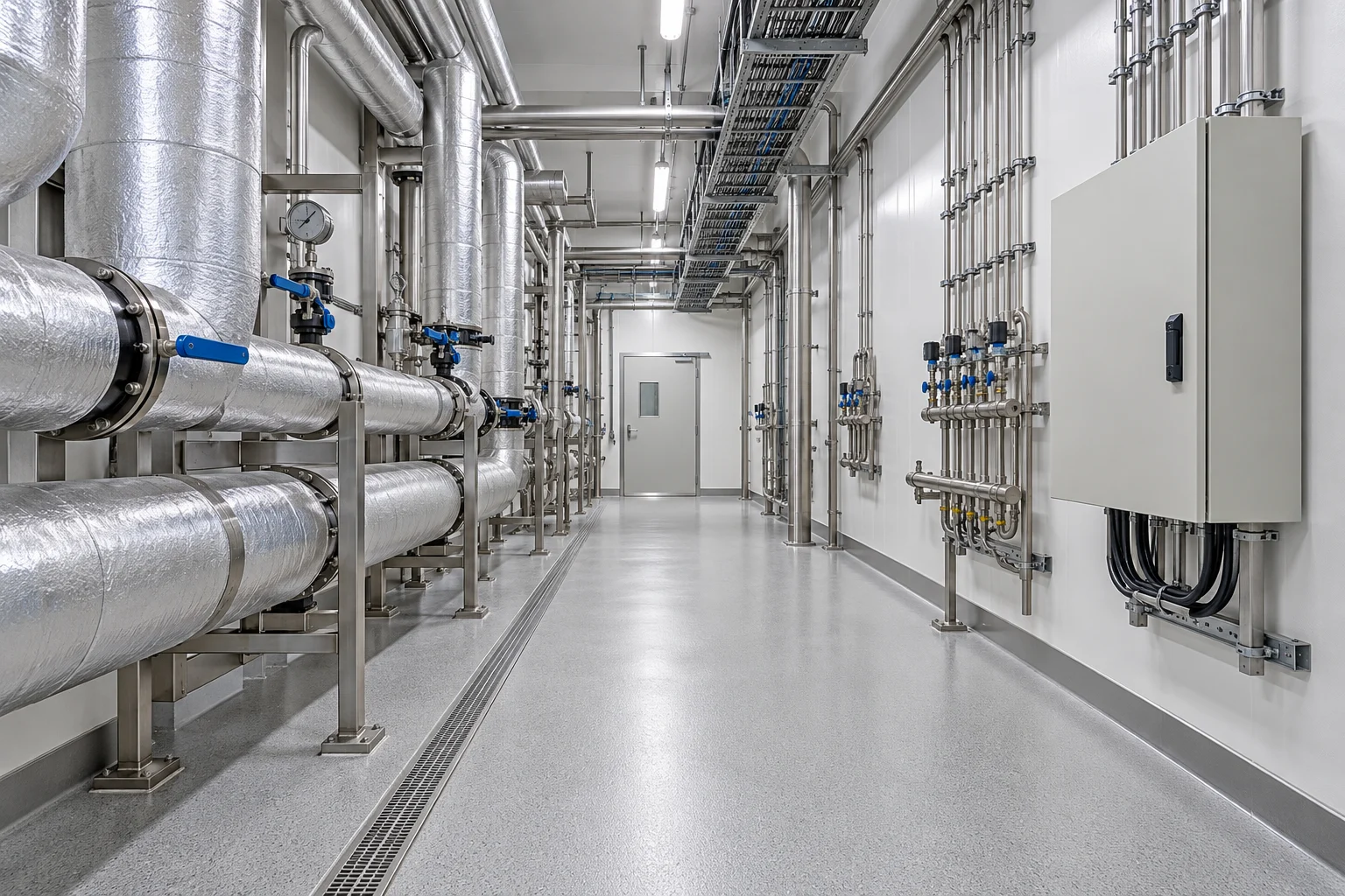
DPS publishes process engineering, configured equipment, controls and installation / integration services. The source links establish relevant scope. The amounts, time changes, resource reductions and returns here are original hypothetical inputs, not achieved DPS customer results.
Swipe horizontally to compare all columns ↔
| Decision | Targeted intervention | Broader replacement / new operation |
|---|---|---|
| Constraint | A measured gap can be corrected within retained assets. | The verified operating envelope cannot meet product, demand or reliability needs. |
| Cost scope | Include engineering, interfaces, shutdown, commissioning and retained-asset risk. | Include all new systems, site / facility work, OEMs, utilities, ramp and working capital. |
| Benefit | Only incremental contribution and genuinely avoided costs versus the current operation. | Demand-supported contribution less the full additional operating cost versus the agreed alternative. |
| Acceptance | Verify the changed duty and its effect on the complete line. | Verify the integrated new train and the owner’s readiness to operate. |
Prepare the information below, export the assumptions you have modeled, and discuss the unknowns with DPS. An unmeasured input is a question to resolve, not a reason to invent precision.
Checklist and model data stay in this browser until you choose to share them.
Spirax Sarco reports a Scottish distillery flash-steam recovery project with annual savings above £50,000 and an estimated 18-month payback in that historical case. These are supplier-reported site results, not DPS outcomes, current prices or transferable project assumptions.
Guide assumptions reviewed on 26 October 2026. Qualified site / product teams establish regulatory and food-safety requirements; this guide does not prescribe a validated process.

Define a food plant utility design basis using operating events, simultaneous peaks, supply conditions, future capacity and clear package interfaces.

See what separates equipment purchase cost from total installed cost: package boundaries, utilities, installation, controls, testing and exclusions.

Build a food plant interface matrix covering building, process, utilities and controls, using a four-system integration lesson and explicit owners.